ColorCET
Perceptually Uniform Colour Maps
| Summary | Gallery | Download | User Guide | Test Image | Theory |
User Guide
What colour maps do I use? While I have designed many maps I find that I mostly only use a few. This page explains what colour maps I tend to use, when I use them, and why.
Table of Contents
-
Linear colour maps are intended for general use and have colour lightness values that increase or decrease linearly over the colour map's range. Such maps are also known as sequential maps. -

Diverging colour maps are suitable where the data being displayed has a well defined reference value and we are interested in differentiating values that lie above, or below, the reference value. -
Rainbow colour maps are widely used but it is suggested that they be avoided because they have perceptual dead spots and an inconsistent perceptual ordering of colours. -
Cyclic colour maps have colours that are matched at each end. They are intended for the presentation of data that is cyclic such as orientation values or angular phase data. -
Low Contrast colour maps are designed for use with relief shading. The relief shading provides the structural information and the colours provide the data classification information. - Appendix 1: Colour Map Paths in CIELAB Colour Space.
-
Appendix 2: Comparison of CET-L20 / Gouldian with MATLAB's Parula. -
Appendix 3: The Painbow.
Linear colour maps
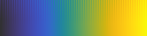
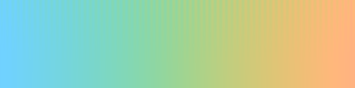
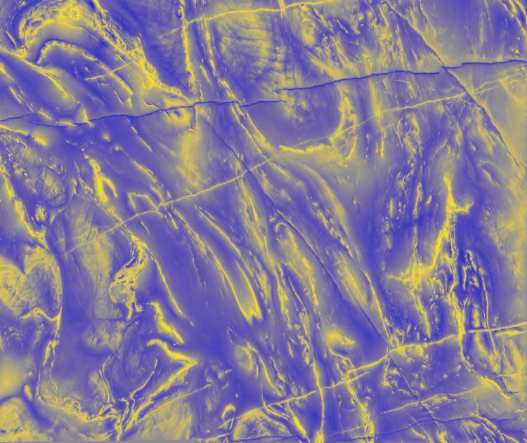
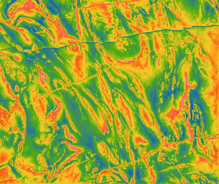
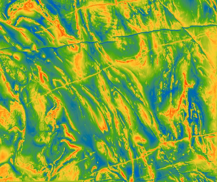
Linear / sequential colour maps are intended for general use and have colour lightness values that increase or decrease linearly over the colour map's range. Generally I use either a grey scale, a heat map, or my (new) favourite, the CET-L20 map which follows a black-blue-green-orange-yellow colour sequence.
Renderings of Magnetic Data Over the Yilgarn in Western Australia
 |
 |
 |
 |
| CET-L01 | CET-L02 |
|---|
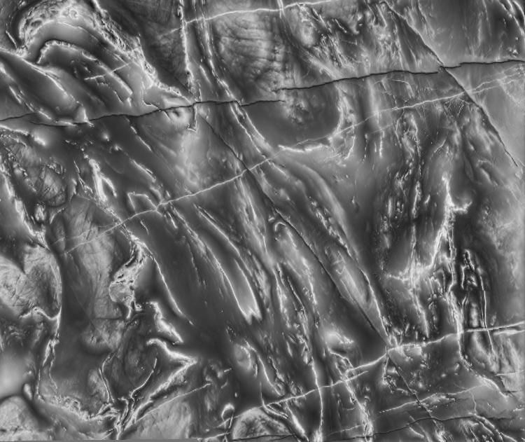
CET-L01 is a grey colour map following a linear lightness profile within CIELAB space. This is slightly different from a linear grey scale in RGB space though the difference is typically hard to discern.
CET-L02 is a grey colour map with slightly reduced contrast starting at a lightness value of 10 and finishing at 95 (rather than 0 and 100). I find that monitors and printers can display this range more reliably and features at the dark and light ends of the colour map are less susceptible to saturation. So, while the image will be rendered with slightly lower contrast, the ability to identify features in the data may be better, especially at the dark end of the scale. I quite often find myself using this map rather than CET-L01.
 |
 |
 |
|
| CET-L03 | CET-L20 / Gouldian |
|---|
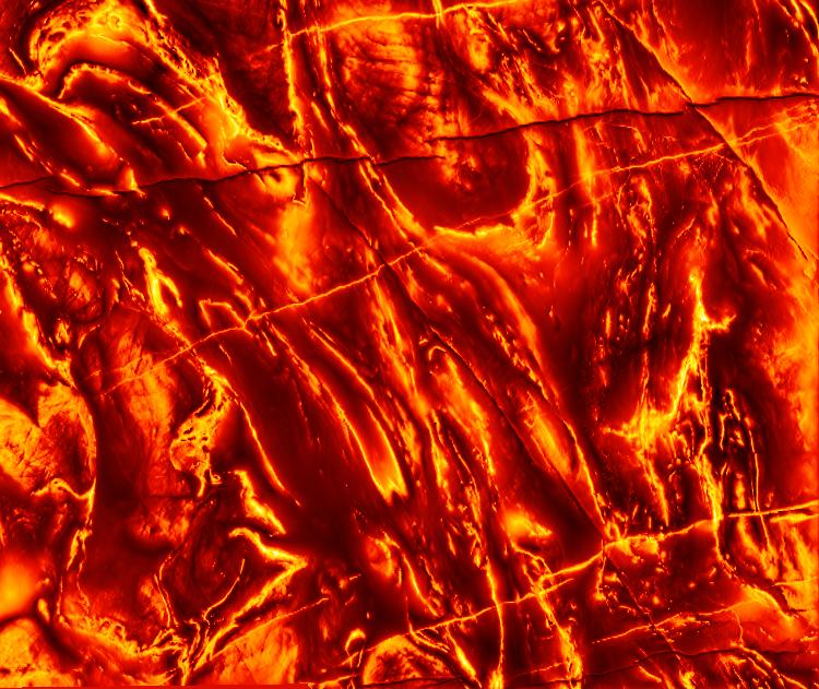
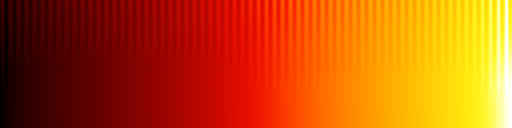
CET-L03 is a perceptually uniform heat map. Typically a heat map is constructed from linear segments along the edges of RGB space from Black to Red to Yellow to White. The sharp direction changes and uniform spacing in RGB space does not produce a perceptually uniform map. To address this CET-L03 is constructed with a smooth path through colour space and is sampled so that the rate of lightness change is constant over the whole map. I have to thank James Bednar who kept pushing me to tweak the map into its final form presented here.
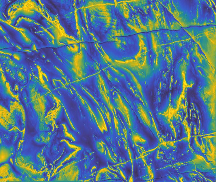
I rather like CET-L20, it is now my default map. I like it so much that I have given it a name, 'Gouldian'. The aim was to produce a colourful map that spans a good range of lightness values. It was influenced by MATLAB's 'Parula' colour map but 'Parula' has some deficiencies that I wanted to overcome. The challenge is to find a colourful path through colour space, from dark to light, that is also a harmonious colour sequence. A heat map achieves this by following a path up the red and yellow side of colour space. CET-L20 starts with a 'cooler' path from black through blue and green transitioning to a hotter sequence of orange to yellow. Each of the colours in the map is reasonably balanced with no single colour dominating the others too much. It took me a while adjusting it until I was satisfied with the result. It works very much better than 'Parula'. See this discussion on the design of this map and its comparison with Parula.
Rendering Issues
Some packages will, by default, scale your data so that a small percentage of
data values will be saturated at the upper and lower ends of your colour map.
Sometimes this is very useful, but sometimes it is not. It is worthwhile
making yourself aware of what your package does by default so that you get the
maximum out of your data.
Diverging colour maps
Diverging colour maps are used where the data being displayed has a well defined reference value and we are interested in differentiating values that lie above, or below, the reference value.
A challenge in designing these maps is that they generally have a lightness gradient reversal at the centre. For example a blue - white - red map increases in lightness going from blue to white and then decreases in lightness as it goes from white to red. This reversal at the centre produces a local region where the lightness gradient is effectively zero. This creates a perceptual dead spot where it will be hard to see features in your data. However, at the same time, the gradient reversal induces a visual feature within the colour map that is independent of the underlying data. Thus it is possible to simultaneously induce both type 1 and type 2 errors at the centre. To avoid creating a false feature at the center I apply a small degree of smoothing to the gradient reversal. However, the price one pays is that this increases the perceptual dead spot very slightly. Be mindful of these issues when interpreting data that is rendered with a diverging colour map.
The three maps I tend to use CET-D01, CET-D07 and CET-D13. For comparison they are shown here using the Yilgarn aeromag data but note this data has no central reference value of interest that would make the use of a diverging map particularly relevant.
 |
 |
|
 |
| CET-D01 | CET-D13 |
|---|
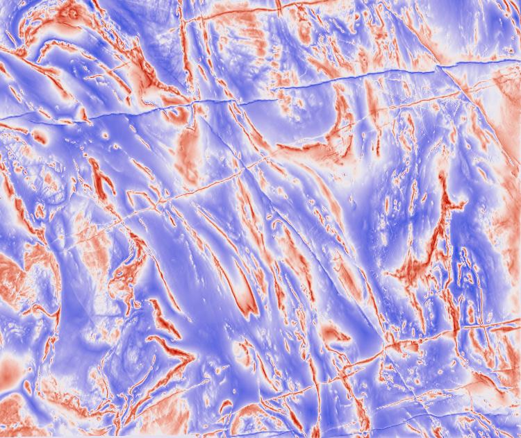
CET-D01 is a classic blue-white-red diverging map. Note however, unlike many vendor maps, the blue and red are matched in lightness and chroma so that the map is perceptually symmetric.
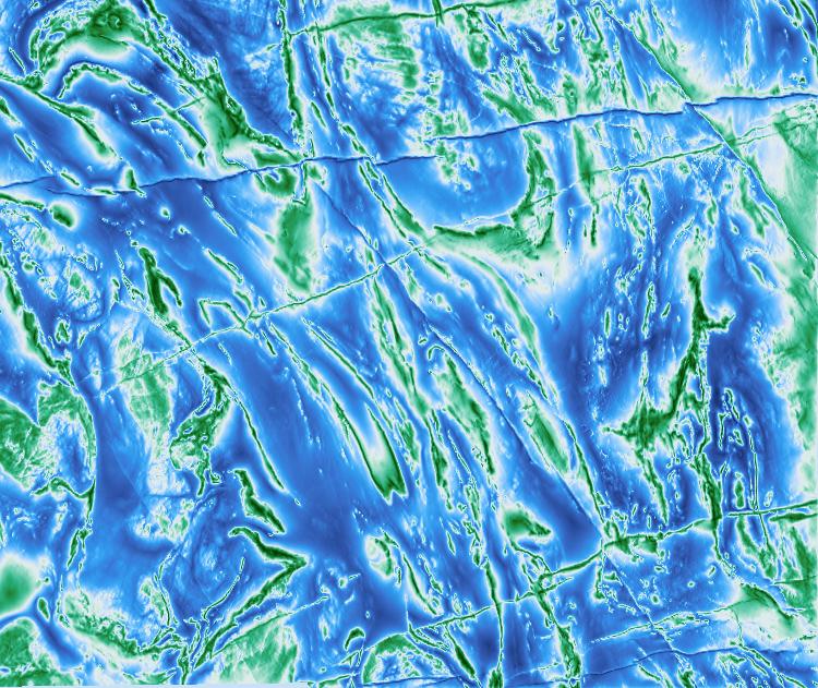
CET-D13 is an attractive diverging map with the blue and green matched for lightness and chroma to achieve perceptual symmetry. I would like to acknowledge that this map was inspired by a similar design by Francesca Samsel at The University of Texas at Austin. I would never have thought to combine blue and green in a diverging map. You can find some of her very attractive and interesting visualisation work at sciviscolor.org
Notice how 'crisp' the renderings above look compared to the renderings using linear colour maps. A diverging map that goes from a dark colour to white to a dark colour again can have a lightness gradient that is up to twice that of a linear colour map. Thus structures in the data are amplified. This is a useful feature of diverging maps, but do be mindful of the perceptual dead point at white.
 |
 |
| CET-D07 |
|---|
In designing a linear-diverging map one is heavily constrained by the colour space gamut. For perceptual symmetry the end point colours must have equal chroma and be equally lighter/darker than the central grey value. Basically, there is not much option but to use this colour sequence.
Rendering Issues with Diverging Maps
Many visualisation packages do not provide specific tools for ensuring your
data is correctly rendered with a diverging colour map. Some, such as
GMT
and QGIS provide specific controls to
allow you to correctly associate specific values with the end points of your
colour map and thus ensure the mid point of a diverging map is correctly
associated with the datum value in your image.
However, many visualisation packages simply scale your data so that the minimum and maximum values in your data are associated with the first and last elements in your colour map. So, for your data to be rendered correctly, you may have to insert a specific value into your image, say in the first pixel, so that the minimum and maximum values of your data result in the appropriate association of colours to your data values.
However, ensuring your image has the appropriate minimum and maximum values may not be enough. As mentioned earlier some packages will, by default, scale your data so that a small percentage of data values will be saturated at the upper and lower ends of your colour map. Thus, you will need to additionally turn this off to obtain a correct rendering.
I have written some MATLAB and Julia code which you may find useful for rendering diverging data.
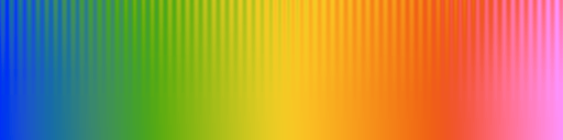
Rainbow colour maps
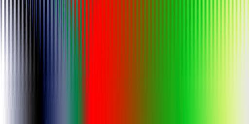
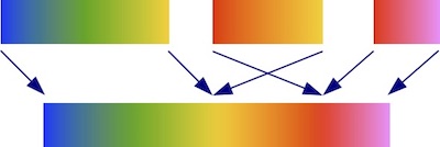
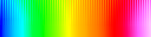
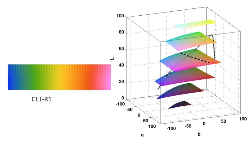
Please avoid using rainbow colour maps, they have a number of problems. They follow a contrived path through CIELAB space that has reversals in the lightness gradient at yellow and red. As with diverging maps these reversals create perceptual dead spots that, at the same time, can also induce false features. The other problem with the lightness gradient reversals is that it produces some confusion in the perceptual ordering of colours. We intuitively accept that yellow is 'greater' than green which, in turn, is 'greater' than blue. However we also typically accept that yellow is 'greater' than red (as in a heat map) but with a rainbow map the opposite ordering applies. In the figure below you can see how a rainbow map can be thought of being composed of three linear maps but with the central heat map confusingly inserted back-to-front.
Thus, I hope you now agree that rainbow colour maps are problematic. However, they are attractive and perhaps can have a legitimate use where the main aim is to differentiate data values rather than communicate a data ordering. Please be mindful of their problems when interpreting data that has been rendered with such maps.
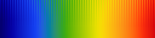
The colour maps presented here are perhaps the 'least worst' rainbow colour maps I can generate. Their paths through colour space are more subdued than is typically used and the lightness reversals at yellow and red have been smoothed to reduce the perception of false anomalies at these points. However, be wary of the slight loss of perceptual contrast at these points. I prefer CET-R2 as it has only one lightness gradient reversal.
 |
 |
|
 |
| CET-R1 | CET-R2 |
|---|
A key feature of these maps is that the colour map path does not go through cyan. Most vendor rainbow maps include cyan and this creates a large perceptual dead zone in the green section. This arises because the colour sequence cyan-green-yellow has very little variation in lightness. It is the lightness variation in colours that produces perceptual contrast.
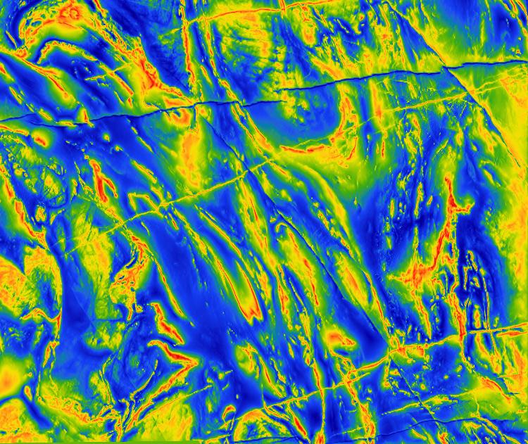
What can go wrong...
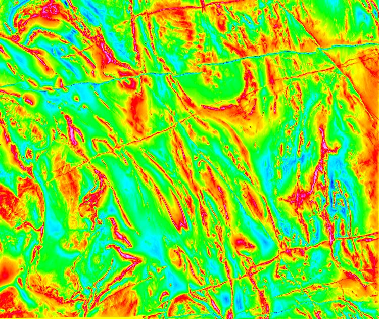
Shown below is the result of rendering the image with a typical vendor map that exhibits a large perceptual dead zone at green, a smaller dead zone at red, and false features at cyan and yellow. So much information has been lost. Note how the green regions reveal no structure. A disaster!! Be very wary of using rainbow colour maps. (This is the default colour map of a widely used geophysics package.)
 |
 |
| Vendor Map |
|---|
Beware of vivid colours
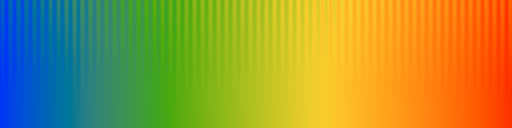
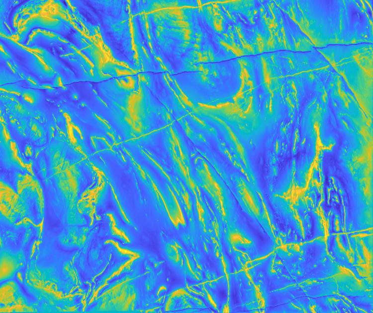
People have commented that the colours in CET-R1 and CET-R2 are a bit dull. In an attempt to address this I created CET-R4. At first sight the colour map looks quite attractive. However, the risk with using a colour map with several very distinct colours is that visually you end up segmenting the image into separate regions corresponding to those distinct colours. It is important that the segmentation should be a function of the structure in the data, not the colours in the colour map.
In the image below the eye is drawn towards the 'islands' of red and yellow in the green-blue background. The overall underlying continuous structure of the data is somewhat obscured. Compare this to the rendering of the data using CET-L1 or CET-L20 above. Using a colour map with a more gradual and continuous transition of hues prevents this problem from occurring. This issue is particularly problematic on smooth images with low spatial frequencies.
 |
 |
| CET-R4 |
|---|
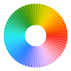
Cyclic colour maps
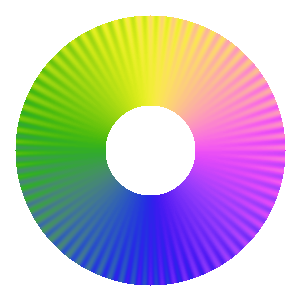
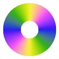
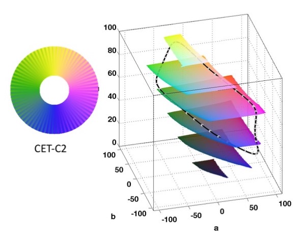
Effective presentation of cyclic data such as orientation information or angular phase values can be quite difficult. A colour map that is often employed for this is the fully saturated hue circle from the HSV colour space.
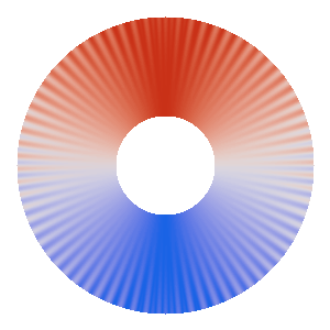
Thus, the challenge is to design a colour map that passes through four distinct colours in a harmonious combination and also has good perceptual contrast. This is very difficult. I think my best effort is CET-C2. (Though now I am preferring CET-C7, see below). The map features four distinct colours, blue, magenta, yellow and green. However I am not entirely satisfied with it as the width of the yellow section is a bit small. The other map I tend to use is CET-C4 which works well if one simply wants to indicate positive and negative phase angles.
 |
 |
| CET-C2 | CET-C4 |
|---|
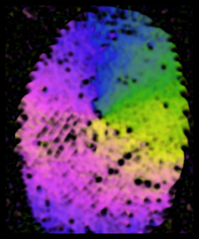
A difficulty with rendering orientation information is that it is often accompanied by amplitude information which we would like to render as well. A common approach is to desaturate the colours towards black, or white, to indicate a low amplitude. In other cases we may only be interested in whether the orientation information is well defined/valid in which case the invalid regions can be masked out.
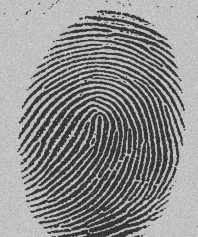
For the fingerprint image below the ridge orientations have been rendered with CET-C2. Areas where orientation information is undefined have been masked out as black. Notice here we are interested in orientation information which has a period of pi (as distinct from direction information with a period of 2pi).
 |
 |
 |
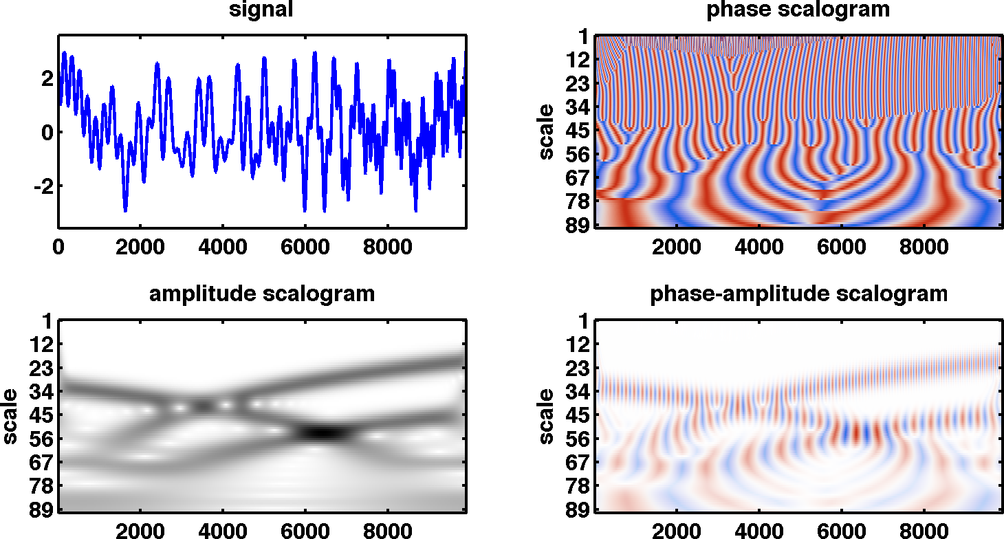
Below we have a scalogram of a 1D signal. This provides local phase and amplitude information as a function of scale at every point along the signal. Here CET-C4 has been used as we only need to identify positive and negative phase angles to interpret the data. The phase-amplitude scalogram uses desaturation of the colours towards white to indicate low amplitude.
A couple of recent maps
CET-C6 is a six-colour map. I have attempted to construct a modified colour circle where the primary colours of red, green and blue have been adjusted so that they are matched in lightness at 50. Similarly, the secondary colours have been adjusted to a lightness value of 90. Thus the lightness values zig-zag up and down between 50 and 90 as we go around the circle. Unfortunately magenta ends up with little chroma at a lightness of 90 due to gamut constraints. However, overall I think it works quite well.
CET-C7 is now my preferred four-colour map. It consists of a zig-zag path through LAB space of yellow - magenta - cyan - green - yellow. The colours are well balanced over the quadrants and are reasonably harmonious.
|
 |
| CET-C6 | CET-C7 |
|---|
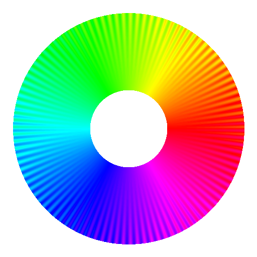
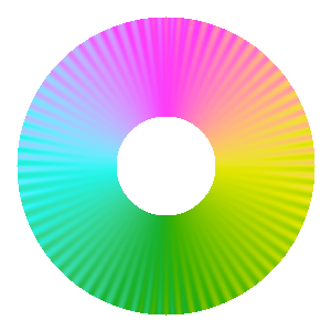
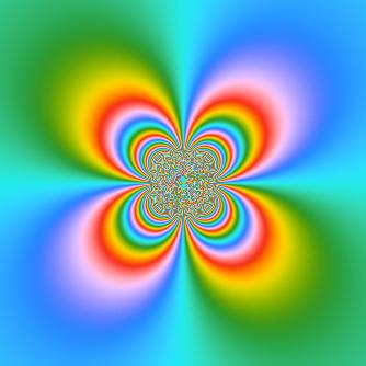
Shown below are the phase angle plots of exp(1/Z2) rendered with the new maps, and also CET-C4 and the standard colour circle for comparison. Perhaps, in the end, CET-C4 is the easiest to interpret and the most informative. I think you will agree that the rendering with the standard colour circle is truly awful!
 |
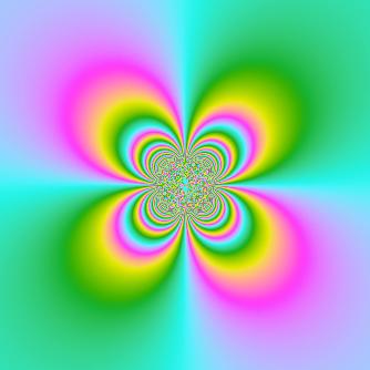 |
| CET-C6 | CET-C7 |
|---|---|
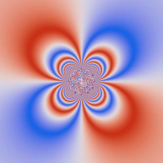 |
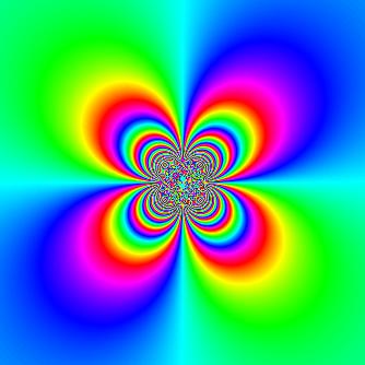 |
| CET-C4 | Standard Colour Circle |
Rendering Issues with Cyclic Maps
Generally there is little provision for controlling the rendering of cyclic
data in visualisation packages. Ideally you want to be able to specify the
period of the data, pi, 2pi, 7 days, etc so that the data values can be mapped
to the colours modulo the period. In addition one may want to apply a
circular shift to the colour map to associate a particular colour with a
reference point in the data cycle (as was done in the fingerprint
example). Finally one may want to use amplitude data to mask the resulting
image or to desaturate the colours towards black or white. I have written
some
MATLAB
and Julia
code which you may find useful.
Colour maps for relief shading
I am quite a fan of relief shading. The use of colour in conjunction with relief shading can provide a powerful enhancement to the perception of shape induced by the shading. However, effective use of relief shading does require some care.
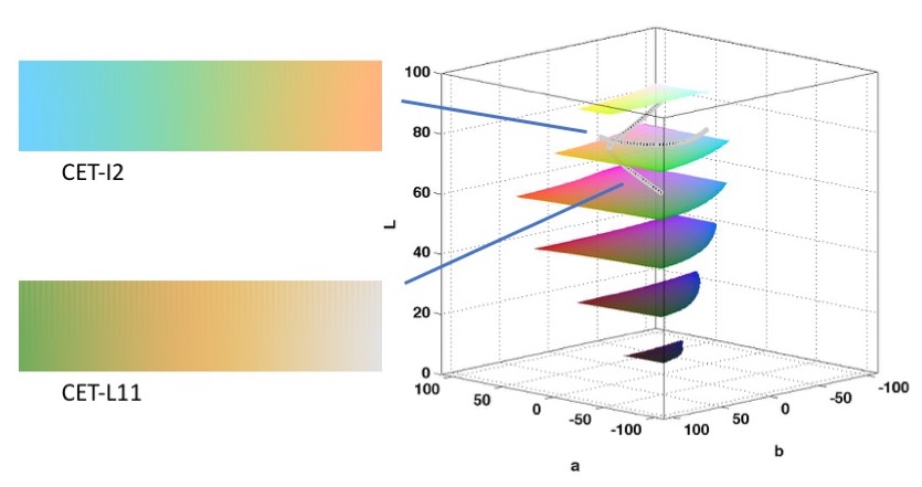
The maps I tend to use in conjunction with relief shading are: CET-L11, a 'geographic' style map, DET-D09, a lighter version of CET-D01, and CET-I2, a light isoluminant (constant lightness) colour map.
Firstly, a consideration when combining colour with relief shading is to ensure that the colour map does not interfere with the perception of features induced by the shading. If the colour map has a wide range of lightness values then potentially this may interfere with the relief shading. Fortunately in practice this is rarely a problem and, indeed, a grey scale map can even work quite effectively with relief shading. However, as a general guide, colour maps for use with relief shading should be of lower contrast so that interaction with the shading is minimal. In addition the colour map should be lighter than otherwise normal because the application of the relief shading will make the overall image darker.
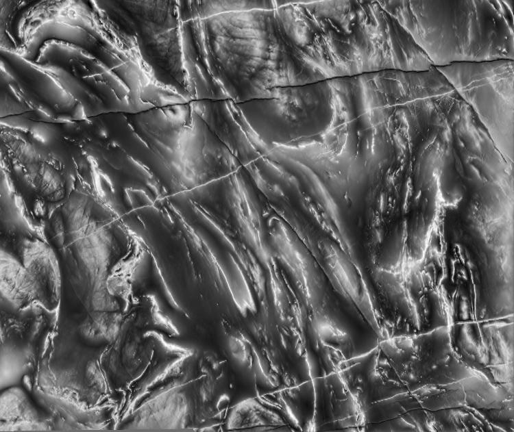
Shown below is a elevation map rendered with the low contrast map CET-L11. On its own this image does not convey the structure of the elevation map very well. However, when this is then applied multiplicatively to the shading of the elevation map to produce the final image on the right we obtain a very informative image. Notice how the final result is greater than the sum of its parts, we have an amplification of the perception of 3D. When a shading pattern is combined with a coloured image such that the colour gradients are not aligned with the shading gradients an amplification of the 3D shading perception will be obtained. For a description of this effect see Kingdom (2003).
 |
x | 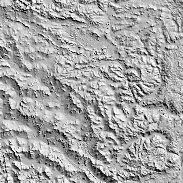 |
= | 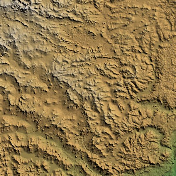 |
| CET-L11 |
|---|
Note that in this example the shading pattern is applied to the colour image multiplicatively. To achieve the perception of a coloured surface being shaded the luminance of the colours need to be modulated by the relief shading. Be wary of some GIS implementations where it is only possible to combine a shading image with a colour image via a transparency blending of the two images, a weighted sum. This is the wrong mechanism to use and will not result in any amplification of the perception of 3D.
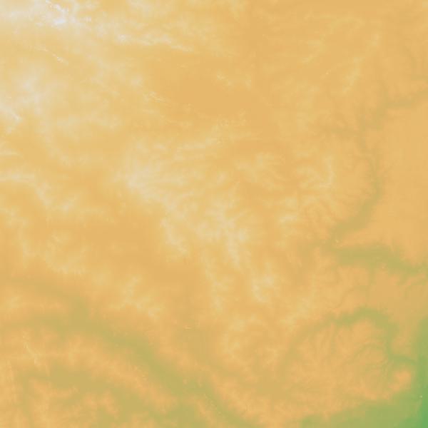
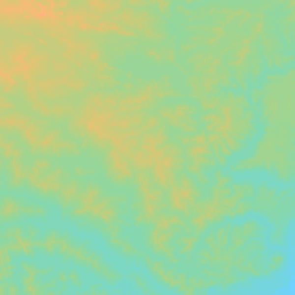
In the example below the elevation image has been rendered with the isoluminant colour map CET-I2. That is, the colours in the map are of constant lightness. With such a colour map there is very little perceptual contrast and fine scale features become effectively invisible. However, when combined with the relief shading we obtain a useful image. In this case the use of an isoluminant colour map means that there is no interaction between the colours and the shading.
 |
x | |
= | 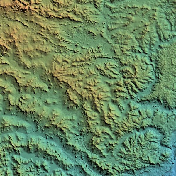 |
| CET-I2 |
|---|
An important advantage of combining relief shading with an image that has been derived from the data is that it allows the communication of overall data properties, metric information, in addition to the form and structure that is provided by the shading. With just a raw grey scale relief image you only get a sense of the local surface normal information, you have no sense of the absolute data values. If the data range is very large this can be useful as the relief shading acts a form of dynamic range reduction allowing small scale features to still be seen within an arbitrarily large range of data values. However, in other cases the loss of any sense of absolute data value can be a disadvantage. Overlaying an image derived from the data values overcomes this problem and allows the best of both worlds.
In other applications it may be useful to combine the colour information from one data set with the shading of a second data set. Thus, the information from two data sets can be simultaneously presented in the one image.
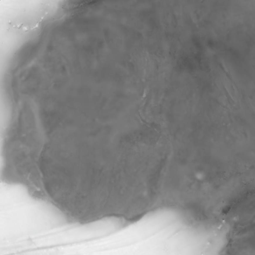
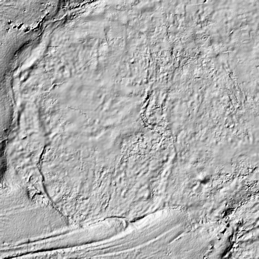
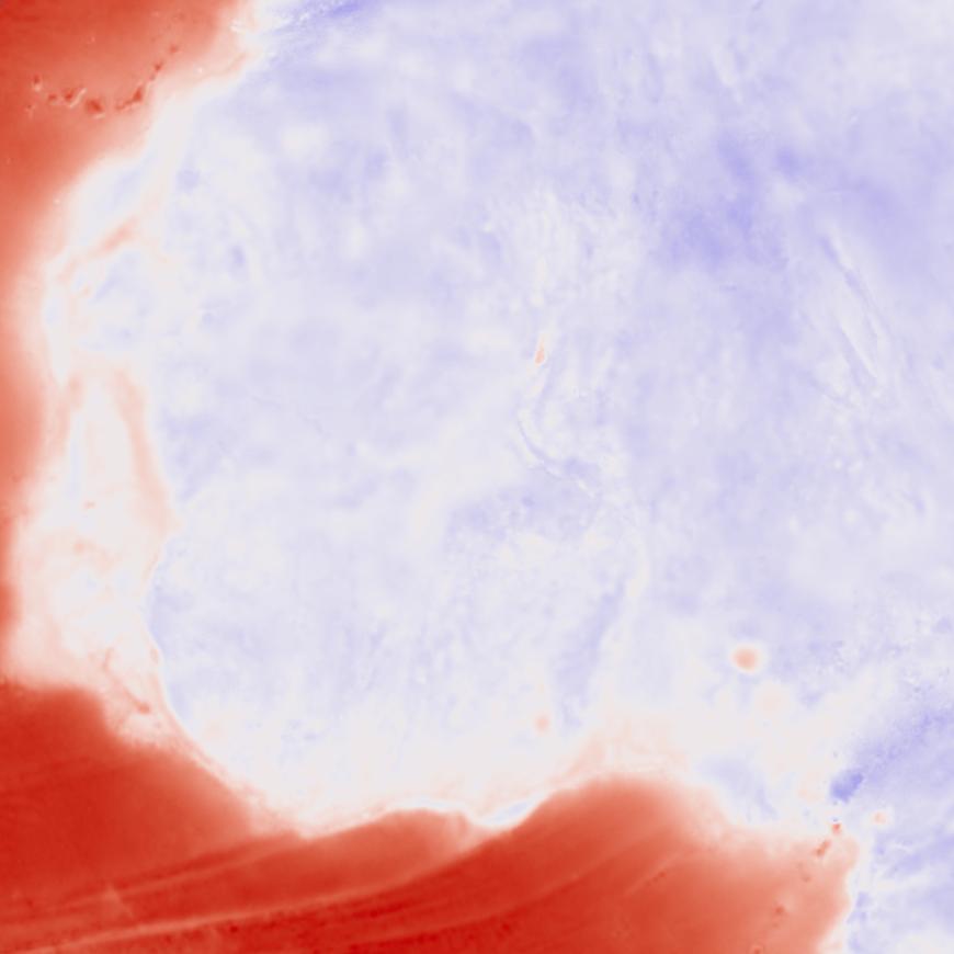
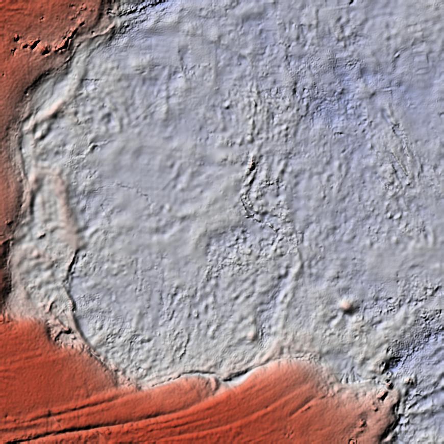
Residual Gravity Image of West Africa
 |
 |
 |
 |
 |
|
| CET-D09 |
|---|
In the top-left we have a grey scale rendering of the data, not much detailed structure can be seen. The relief shaded image shown top-right allows small scale structures to be identified readily. However, it is hard to get a sense of the magnitude of the deviation of features above and below zero. In the bottom-left we have a rendering of the data with CET-D09, a lighter version of CET-D01. As with the grey scale rendering not much detail can be seen and the perceptual flat spot in the white regions is particularly noticeable. However, when this image is multiplicatively combined with the relief shading image the fine structures in the data can be seen in conjunction with the magnitude and polarity of the data values.
Reference:F. A. Kingdom, "Color brings relief to human vision," Nature Neuroscience, vol. 6, no. 6, pp. 641-644, June 2003.
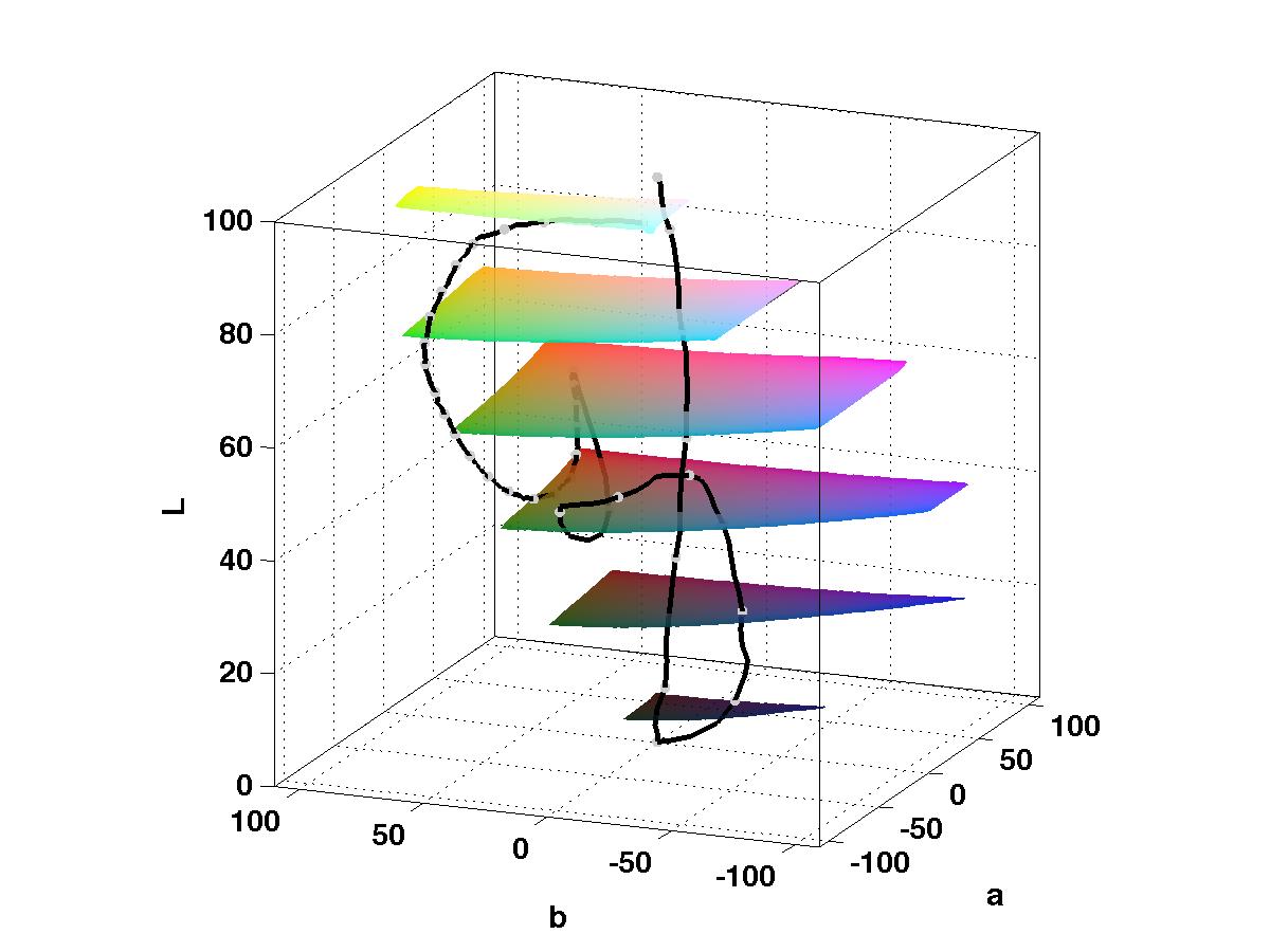
Appendix 1: Colour Map Paths in CIELAB Colour Space
It is instructive to see the paths through colour space of different colour maps. Rather than display the paths in RGB colour space I prefer to use CIELAB colour space, also known as CIE L*a*b*. The three axes of this colour space are:
- L* the lightness value varying from 0 to 100.
- a* the green-red axis.
- b* the yellow-blue axis.
To illustrate the differences between the colour spaces shown below is the colour map path for CET-L03 in RGB space on the left and CIELAB on the right.
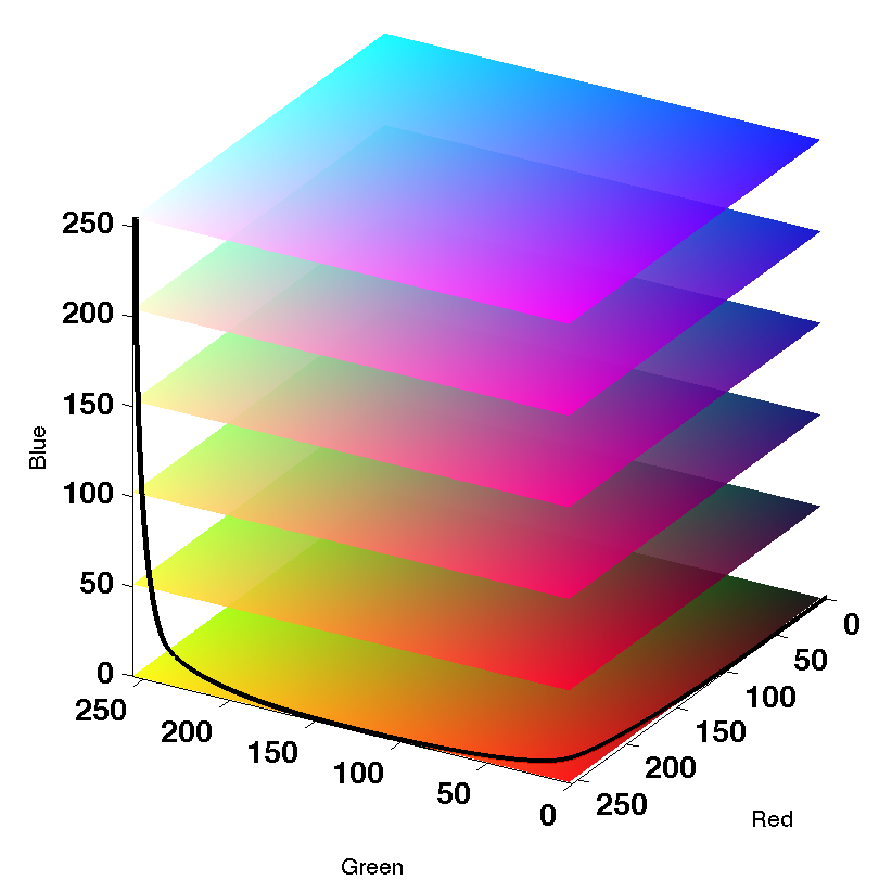 |
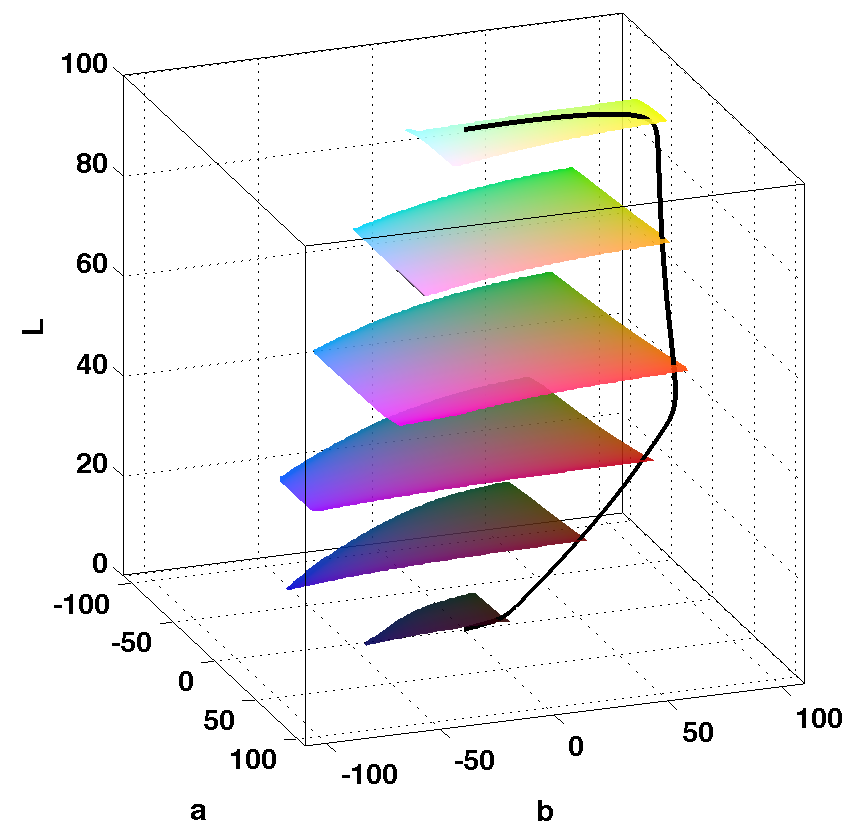 |
| RGB | CIELAB |
|---|
Sampling the path through CIELAB space such that the change in the L* component is constant at each step produces the heat colour map CET-L3 that we see at the top.
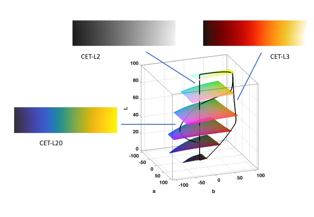
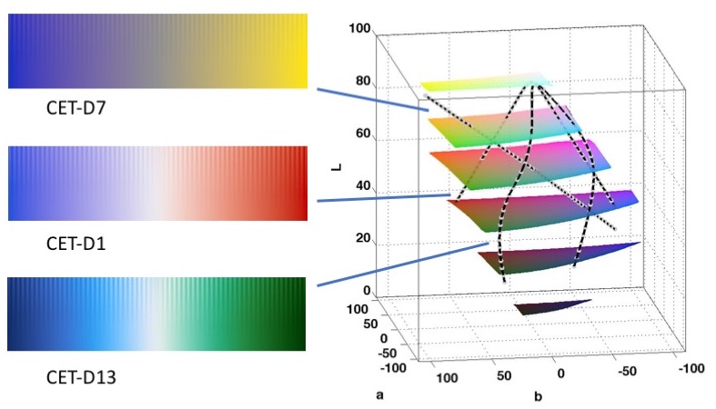
The fact that CIELAB organises colours in terms of their lightness allows us to see and understand the characteristics of different colour maps.
Here are the paths in CIELAB space of some of the colour maps shown above
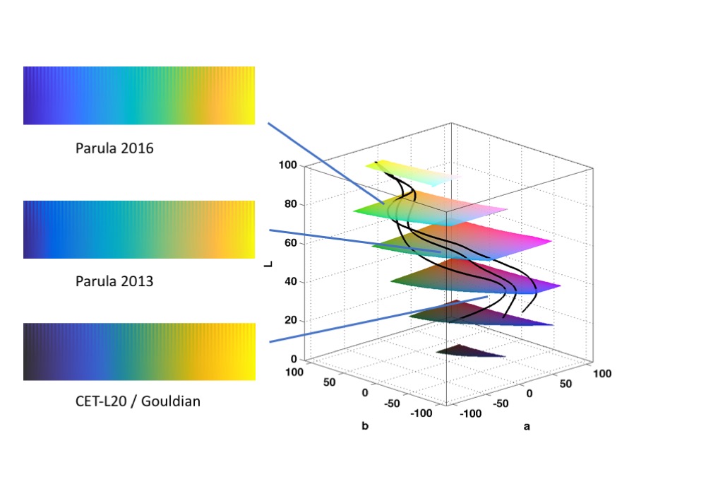
Appendix 2: Comparison of CET-L20 / Gouldian with MATLAB's Parula
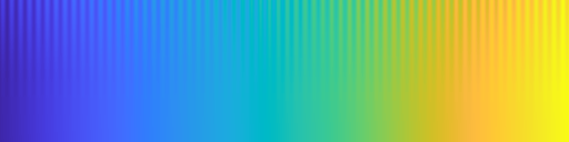
In 2013 MATLAB introduced Parula as their new default colour map to replace 'jet'. When I evaluated the colour map by computing the colour lightness differences along the map and also by viewing it on my test image I observed that it had a high perceptual contrast at the lower end of the range but suffered with poor contrast in the mid section from cyan to orange. The colour map was revised a bit in 2016 which improved things slightly but the transition in hue from green to orange ended up being slightly more abrupt, often appearing as a hard boundary on some images. Overall I did not think the colour map worked very well. However, I thought the colour transition sequence was interesting and I set out to design an improved map along these lines.
The final result was a path through colour space that was smoother and did not attempt to include cyan. The path maintains a more uniform slope upwards in CIELAB space which prevents the abrupt transition from green to orange that Parula suffers from. I also made the map start at a very dark grey (with a lightness of 20) before transitioning to blue. This added an extra 'colour' to the map and reduced the width of the blue section so that blue did not overly dominate the colour scheme.
|
 |
|
|
| CET-L20 / Gouldian | Parula 2016 |
|---|
Appendix 3: The Painbow
xkcd has produced a wonderful example of the colour map from hell, the Painbow!
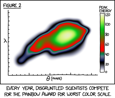
For fun here is the Painbow rendered on the test image and a plot of its wild path through LAB colour space.